Ibis 聲明式多引擎資料堆疊
TL;DR
I recently came across the Ju Data Engineering Newsletter by Julien Hurault on the multi-engine data stack. The idea is simple; we'd like to easily port our code across any backend while retaining the flexibility to grow our pipeline as new backends and features are developed. This entails in at least the following high-level workflows:
- Offloading part of a SQL query to serverless engines with DuckDB, polars, DataFusion, chdb etc.
- Right-size pipeline for various development and deployment scenarios. For example, developers can work locally and ship to production with confidence.
- Apply database style optimizations to your pipelines automatically.
In this post, we dive into how we can implement the multi-engine pipeline from a programming language; Instead of SQL, we use propose using a Dataframe API that can be used for both interactive and batch use-cases. Specifically, we show how to break up our pipeline into smaller pieces and execute them across DuckDB, pandas, and Snowflake. We also discuss the advantages of a multi-engine data stack and highlight emerging trends in the field.
The code implemented in this post is available on GitHub^[In order to quickly try out repo, I also provide a nix flake]. The reference work in the newsletter with original implementation is here.
Overview
Multi-engine data stack pipeline works as follows: Some data lands in an S3 bucket, gets preprocessed to remove any duplicates and then loaded into a Snowflake table, where it is transformed further with ML or Snowflake specific functions^[Please note we do not go into implementing the types of things that might be possible in Snowflake and assume that as a requirement for the workflow]. The pipeline takes orders as parquet files that get saved into landing location, are preprocessed and then stored at the staging location in an S3 bucket. The staging data is then loaded in Snowflake to connect downstream BI tools to it. The pipeline is tied together by SQL dbt with one model for each backend and the newsletter chooses Dagster as the orchestration tool.
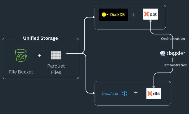
Today, we are going to dive into how we can convert our pandas code to Ibis expressions, reproducing the complete example for Julien Hurault's multi engine stack example 1. Instead of using dbt Models and SQL, we use ibis and some Python to compile and orchestrate SQL engines from a shell. By rewriting our code as Ibis expressions, we can declaratively build our data pipelines with deferred execution. Moreover, Ibis supports over 20 backends, so we can write code once and port our ibis.exprs to multiple backends. To further simplify, we leave scheduling and task orchestration2 provided by Dagster, up to the reader.
Core Concept of Multi-Engine Data Stack
Here are the core concepts of the multi-engine data stack as outlined in Julien's newsletter:
- Multi-Engine Data Stack: The concept involves combining different data engines like Snowflake, Spark, DuckDB, and BigQuery. This approach aims to reduce costs, limit vendor lock-in, and increase flexibility. Julien mentions that for certain benchmark queries, using DuckDB could achieve a significant cost reduction compared to Snowflake.
- Development of a Cross-Engine Query Layer: The newsletter highlights advancements in technology that allow data teams to transpile their SQL or Dataframe code from one engine to another seamlessly. This development is crucial for maintaining efficiency across different engines.
- Use of Apache Iceberg and Alternatives: While Apache Iceberg is seen as a potential unified storage layer, its integration is not yet mature to be used in a dbt project. Instead, Julien has opted to use Parquet files stored in S3, accessed by both DuckDB and Snowflake, in his Proof of Concept (PoC).
- Orchestration and Engines in PoC: For the project, Julien used Dagster as the orchestrator, which simplifies the job scheduling of different engines within a dbt project. The engines combined in this PoC were DuckDB and Snowflake.
Why DataFrames and Ibis?
While the pipeline above is nice for ETL and ELT, sometimes we want the power of a full programming language instead of a Query Language like SQL e.g. debugging, testing, complex UDFs etc. For scientific exploration, interactive computing is essential as data scientists need to quickly iterate on their code, visualize the results, and make decisions based on the data.
DataFrames are such a data structure: DataFrames are used to process ordered data and apply compute operations on it in an interactive manner. They provide the flexibility to be able to process large data with SQL style operations, but also provides lower level control to edit cell level changes ala Excel Sheets. Typically, the expectation is that all data is processed in-memory and typically fits in-memory. Moreover, DataFrames make it easy to go back and forth between deferred/batch and interactive modes.
DataFrames excel^[no pun intended] at enabling folks to apply user-defined functions and releases a user from the limitations of SQL i.e. You can now re-use code, test your operations, easily extend relational machinery for complex operations. DataFrames also make it easy to quickly go from Tabular representation of data into Arrays and Tensors expected by Machine Learning libraries.
Specialized and in-process databases e.g. DuckDB for OLAP3, are blurring the boundary between a remote heavy weight database like Snowflake and an ergonomic library like pandas. We believe this is an opportunity for allowing DataFrames to process larger than memory data while maintaining the interactivity expectations and developer feel of a local Python shell, making larger than memory data feel small.
Technical Deep Dive
Our implementation focuses on the 4 concepts presented earlier:
- Multi-Engine Data Stack: We will use DuckDB, pandas, and Snowflake as our engines.
- Cross-Engine Query Layer: We will use Ibis to write our expressions and compile them to run on DuckDB, pandas, and Snowflake.
- Apache Iceberg and Alternatives: We will use Parquet files stored locally as our storage layer with the expectation that its trivial to extend to S3 using s3fs package.
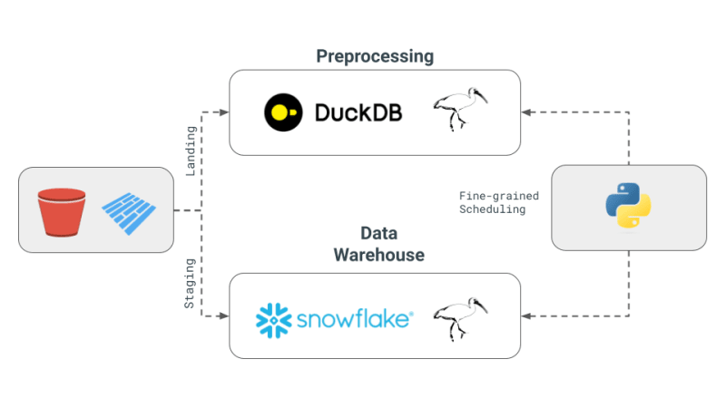
- Orchestration and Engines in PoC: We will focus on fine-grained scheduling for engines and leave orchestration to the reader. Fine-grained scheduling is more aligned with Ray, Dask, PySpark as compared to orchestration frameworks e.g. Dagster, Airflow etc.
Implementing with pandas
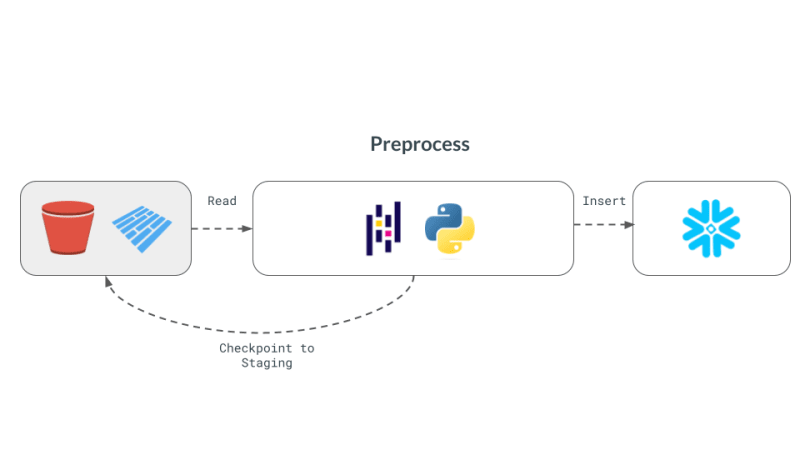
pandas is the quintessential DataFrame library and perhaps provides the simplest way to implement the above workflow. First, we generate random data borrowing from the implementation in the newsletter.
#| echo: false
import pandas as pd
from multi_engine_stack_ibis.generator import generate_random_data
generate_random_data("landing/orders.parquet")
df = pd.read_parquet("landing/orders.parquet")
deduped = df.drop_duplicates(["order_id", "dt"])
The pandas implementation is imperative in style and is designed so the data that can fit in memory. The pandas API is hard to compile down to SQL with all its nuances and largely sits in its own special place bringing together Python visualization, plotting, machine learning, AI and complex processing libraries.
pt.write_pandas(
    conn,
    deduped,
    table_name="T_ORDERS",
    auto_create_table=True,
    quote_identifiers=False,
    table_type="temporary"
)
After de-duplicating using pandas operators, we are ready to send the data to Snowflake. Snowflake has a method called write_pandas that comes in handy for our use-case.
Implementing with Ibis aka Ibisify
One pandas limitation is that it has its own API that does not quite map back to relational algebra. Ibis is such a library that's literally built by people who built pandas to provide a sane expressions system that can be mapped back to multiple SQL backends. Ibis takes inspiration from the dplyr R package to build a new expression system that can easily map back to relational algebra and thus compile to SQL. It also is declarative in style, enabling us to apply database style optimizations on the complete logical plan or the expression. Ibis is a key component for enabling composability as highlighted in the excellent composable codex.
#| echo: false
import pathlib

import ibis
import ibis.backends.pandas.executor
import ibis.expr.types.relations
from ibis import _

from multi_engine_stack_ibis.generator import generate_random_data
from multi_engine_stack_ibis.utils import (MyExecutor, checkpoint_parquet,
                                           create_table_snowflake,
                                           replace_unbound)
from multi_engine_stack_ibis.connections import make_ibis_snowflake_connection


ibis.backends.pandas.executor.PandasExecutor = MyExecutor
setattr(ibis.expr.types.relations.Table, "checkpoint_parquet", checkpoint_parquet)
setattr(
    ibis.expr.types.relations.Table,
    "create_table_snowflake",
    create_table_snowflake,
)
ibis.set_backend("pandas")
p_staging = pathlib.Path("staging/staging.parquet")
p_landing = pathlib.Path("landing/orders.parquet")

snow_backend = make_ibis_snowflake_connection(database="MULTI_ENGINE", schema="PUBLIC", warehouse="COMPUTE_WH")
expr = (
  ibis.read_parquet(p_landing)
  .mutate(
      row_number=ibis.row_number().over(group_by=[_.order_id], order_by=[_.dt]))
  .filter(_.row_number == 0)
  .checkpoint_parquet(p_staging)
  .create_table_snowflake("T_ORDERS")
)
expr
Ibis expression prints itself as a plan that is akin to traditional Logical Plan in databases. A Logical Plan is a tree of relational algebra operators that describes the computation that needs to be performed. This plan is then optimized by the query optimizer and converted into a physical plan that is executed by the query executor. Ibis expressions are similar to Logical Plans in that they describe the computation that needs to be performed, but they are not executed immediately. Instead, they are compiled into SQL and executed on the backend when needed. Logical Plan is generally at a higher level of granularity than a DAG produced by a task scheduling framework like Dask. In theory, this plan could be compiled down to Dask's DAG.
While pandas is embedded and is just a pip install away, it still has much documented limitations with plenty of performance improvements left on the table. This is where the recent embedded databases like DuckDB fill the gap of packing the full punch of a SQL engine, with all of its optimizations and benefiting from years of research that is as easy to import as is pandas. In this world, at minimum we can delegate all relational and SQL parts of our pipeline in pandas to DuckDB and only get the processed data ready for complex user defined Python.
Now, we are ready to take our Ibisified code and compile our expression above to execute on arbitrary engines, to truly realize the write-once-run-anywhere paradigm: We have successfully decoupled our compute engine with the expression system describing our computation.
Multi-Engine Data Stack w/ Ibis
DuckDB pandas Snowflake
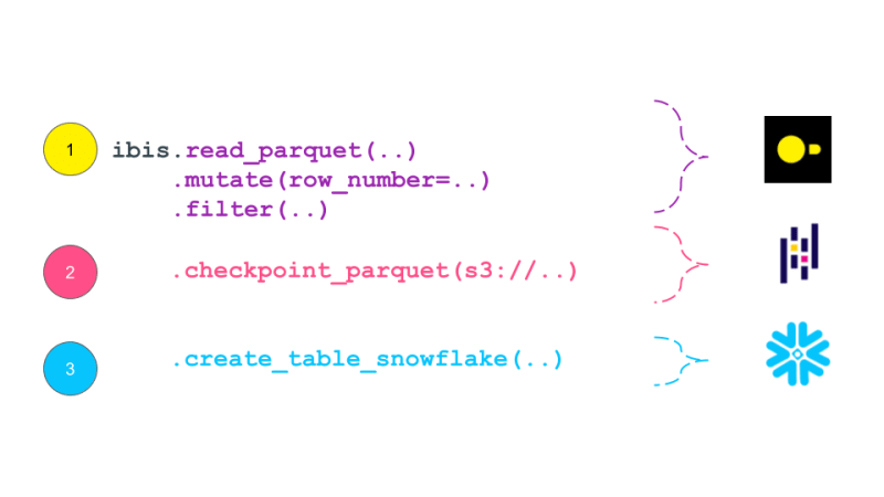
Let's break our expression above into smaller parts and have them run across DuckDB, pandas and Snowflake. Note that we are not doing anything once the data lands in Snowflake and just show that we can select the data. Instead, we are leaving that up to the user's imagination what is possible with Snowflake native features.
Notice our expression above is bound to the pandas backend. First, lets create an UnboundTable expression to not have to depend on a backend when writing our expressions.
schema = {
    "user_id": "int64",
    "dt": "timestamp",
    "order_id": "string",
    "quantity": "int64",
    "purchase_price": "float64",
    "sku": "string",
    "row_number": "int64",
}

first_expr_for = (
    ibis.table(schema, name="orders")
    .mutate(
        row_number=ibis.row_number().over(group_by=[_.order_id], order_by=[_.dt])
    )
    .filter(_.row_number == 0)
)
first_expr_for
Next, we replace the UnboundTable expression with the DuckDB backend and execute it with to_parquet method4. This step is covered by the checkpoint_parquet operator that we added to pandas backend above. Here is an excellent blog that discusses inserting data into Snowflake from any Ibis backend with to_pyarrow functionality.
data = pd.read_parquet("landing/orders.parquet")
duck_backend = ibis.duckdb.connect()
duck_backend.con.execute("CREATE TABLE orders as SELECT * from data")

bind_to_duckdb = replace_unbound(first_expr_for, duck_backend)
bind_to_duckdb.to_parquet(p_staging)
to_sql = ibis.to_sql(bind_to_duckdb)
print(to_sql)
Once the above step creates the de-duplicated table, we can then send data to Snowflake using the pandas backend. This functionality is covered by create_table_snowflake operator that we added to pandas backend above.
second_expr_for = ibis.table(schema, name="T_ORDERS") # nothing special just a reading the data from orders table
snow_backend.create_table("T_ORDERS", schema=second_expr_for.schema(), temp=True)
pandas_backend = ibis.pandas.connect({"T_ORDERS": pd.read_parquet(p_staging)})
snow_backend.insert("T_ORDERS", pandas_backend.to_pyarrow(second_expr_for))
Finally, we can select the data from the Snowflake table to verify that the data has been loaded successfully.
third_expr_for = ibis.table(schema, name="T_ORDERS") # add you Snowflake ML functions here
third_expr_for
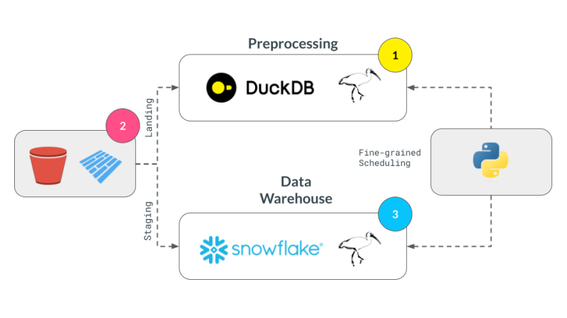
We successfully broke up our computation in pieces, albeit manually, and executed them across DuckDB, pandas, and Snowflake. This demonstrates the flexibility and power of a multi-engine data stack, allowing users to leverage the strengths of different engines to optimize their data processing pipelines.
Acknowledgments
I'd like to thank Neal Richardson, Dan Lovell and Daniel Mesejo for providing the initial feedback on the post. I highly appreciate the early review and encouragement by Wes McKinney.
Resources
- The Road to Composable Data Systems
- The Composable Codex
- Apache Arrow
- Multi-Engine Data Stack Newsleter v0 v1
- Ibis, the portable dataframe library
- dbt Docs
- Dagster Docs
- LanceDB
- KuzuDB
- DuckDB
-
In this post, we have primarily focused on v0 of the multi-engine data stack. In the latest version, Apache Iceberg is included as a storage and data format layer. NYC Taxi data is used instead of the random Orders data treated in this and v0 of the posts. ↩
-
Orchestration Vs fine-grained scheduling: ↩
- The orchestration is left to the reader. The orchestration can be done using a tool like Dagster, Prefect, or Apache Airflow.
- The fine-grained scheduling can be done using a tool like Dask, Ray, or Spark.
-
Some of the examples of in-process databases is described in this post extending DuckDB example above to newer purpose built databases like LanceDB and KuzuDB. ↩
-
The Ibis docs use backend.to_pandas(expr) commands to bind and run the expression in the same go. Instead, we use replace_unbound method to show a generic way to just compile the expression and not execute it to said backend. This is just for illustration purposes. All the code below, uses the backend.to_pyarrow methods from here on. ↩
-
 為什麼使用固定定位時,為什麼具有100%網格板柱的網格超越身體?網格超過身體,用100%grid-template-columns 為什麼在grid-template-colms中具有100%的顯示器,當位置設置為設置的位置時,grid-template-colly修復了? 問題: 考慮以下CSS和html: class =“ snippet-code”> ...程式設計 發佈於2025-03-26
 -
 如何使用FormData()處理多個文件上傳?)處理多個文件輸入時,通常需要處理多個文件上傳時,通常是必要的。 The fd.append("fileToUpload[]", files[x]); method can be used for this purpose, allowing you to send multi...程式設計 發佈於2025-03-26
 -
 Python讀取CSV文件UnicodeDecodeError終極解決方法在試圖使用已內置的CSV模塊讀取Python中時,CSV文件中的Unicode Decode Decode Decode Decode decode Error讀取,您可能會遇到錯誤的錯誤:無法解碼字節 在位置2-3中:截斷\ uxxxxxxxx逃脫當CSV文件包含特殊字符或Unicode的路徑逃...程式設計 發佈於2025-03-26
 -
 如何使用Python的請求和假用戶代理繞過網站塊?如何使用Python的請求模擬瀏覽器行為,以及偽造的用戶代理提供了一個用戶 - 代理標頭一個有效方法是提供有效的用戶式header,以提供有效的用戶 - 設置,該標題可以通過browser和Acterner Systems the equestersystermery和操作系統。通過模仿像Chro...程式設計 發佈於2025-03-26
 -
 如何使用不同數量列的聯合數據庫表?合併列數不同的表 當嘗試合併列數不同的數據庫表時,可能會遇到挑戰。一種直接的方法是在列數較少的表中,為缺失的列追加空值。 例如,考慮兩個表,表 A 和表 B,其中表 A 的列數多於表 B。為了合併這些表,同時處理表 B 中缺失的列,請按照以下步驟操作: 確定表 B 中缺失的列,並將它們添加到表的...程式設計 發佈於2025-03-26
 -
 對象擬合:IE和Edge中的封面失敗,如何修復?To resolve this issue, we employ a clever CSS solution that solves the problem:position: absolute;top: 50%;left: 50%;transform: translate(-50%, -50%)...程式設計 發佈於2025-03-26
 -
 如何修復\“常規錯誤:2006 MySQL Server在插入數據時已經消失\”?How to Resolve "General error: 2006 MySQL server has gone away" While Inserting RecordsIntroduction:Inserting data into a MySQL database can...程式設計 發佈於2025-03-26
 -
 如何在其容器中為DIV創建平滑的左右CSS動畫?通用CSS動畫,用於左右運動 ,我們將探索創建一個通用的CSS動畫,以向左和右移動DIV,從而到達其容器的邊緣。該動畫可以應用於具有絕對定位的任何div,無論其未知長度如何。 問題:使用左直接導致瞬時消失 更加流暢的解決方案:混合轉換和左 [並實現平穩的,線性的運動,我們介紹了線性的轉換。...程式設計 發佈於2025-03-26
 -
 如何將多種用戶類型(學生,老師和管理員)重定向到Firebase應用中的各自活動?Red: How to Redirect Multiple User Types to Respective ActivitiesUnderstanding the ProblemIn a Firebase-based voting app with three distinct user type...程式設計 發佈於2025-03-26
 -
 在Java中使用for-to-loop和迭代器進行收集遍歷之間是否存在性能差異?For Each Loop vs. Iterator: Efficiency in Collection TraversalIntroductionWhen traversing a collection in Java, the choice arises between using a for-...程式設計 發佈於2025-03-26
 -
 如何從PHP中的數組中提取隨機元素?從陣列中的隨機選擇,可以輕鬆從數組中獲取隨機項目。考慮以下數組:; 從此數組中檢索一個隨機項目,利用array_rand( array_rand()函數從數組返回一個隨機鍵。通過將$項目數組索引使用此鍵,我們可以從數組中訪問一個隨機元素。這種方法為選擇隨機項目提供了一種直接且可靠的方法。程式設計 發佈於2025-03-26
 -
 eval()vs. ast.literal_eval():對於用戶輸入,哪個Python函數更安全?稱量()和ast.literal_eval()中的Python Security 在使用用戶輸入時,必須優先確保安全性。強大的python功能eval()通常是作為潛在解決方案而出現的,但擔心其潛在風險。本文深入研究了eval()和ast.literal_eval()之間的差異,突出顯示其安全性含義...程式設計 發佈於2025-03-26
 -
 如何在php中使用捲髮發送原始帖子請求?如何使用php 創建請求來發送原始帖子請求,開始使用curl_init()開始初始化curl session。然後,配置以下選項: curlopt_url:請求 [要發送的原始數據指定內容類型,為原始的帖子請求指定身體的內容類型很重要。在這種情況下,它是文本/平原。要執行此操作,請使用包含以下標頭...程式設計 發佈於2025-03-26
 -
 在GO中構造SQL查詢時,如何安全地加入文本和值?在go中構造文本sql查詢時,在go sql queries 中,在使用conting and contement和contement consem per時,尤其是在使用integer per當per當per時,per per per當per. [&&&&&&&&&&&&&&&&默元組方法在...程式設計 發佈於2025-03-26
 -
 如何有效地轉換PHP中的時區?在PHP 利用dateTime對象和functions DateTime對象及其相應的功能別名為時區轉換提供方便的方法。例如: //定義用戶的時區 date_default_timezone_set('歐洲/倫敦'); //創建DateTime對象 $ dateTime = ne...程式設計 發佈於2025-03-26
學習中文
- 1 走路用中文怎麼說? 走路中文發音,走路中文學習
- 2 坐飛機用中文怎麼說? 坐飞机中文發音,坐飞机中文學習
- 3 坐火車用中文怎麼說? 坐火车中文發音,坐火车中文學習
- 4 坐車用中文怎麼說? 坐车中文發音,坐车中文學習
- 5 開車用中文怎麼說? 开车中文發音,开车中文學習
- 6 游泳用中文怎麼說? 游泳中文發音,游泳中文學習
- 7 騎自行車用中文怎麼說? 骑自行车中文發音,骑自行车中文學習
- 8 你好用中文怎麼說? 你好中文發音,你好中文學習
- 9 謝謝用中文怎麼說? 谢谢中文發音,谢谢中文學習
- 10 How to say goodbye in Chinese? 再见Chinese pronunciation, 再见Chinese learning


