Hi , In this blog we will talk about how we can do Raster analysis with ease using h3 indexes.

Objective

For learning, We will do calculation on figuring out how many buildings are there in settlement area determined by ESRI Land Cover. Lets aim of national level data for both vector and raster .

Let's first find the data

Download Raster Data

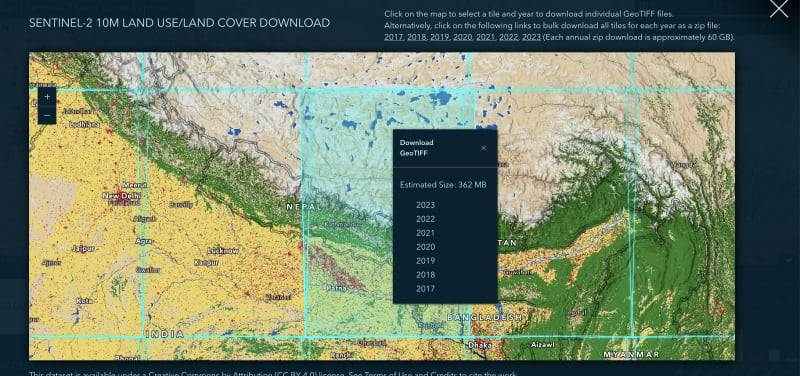
I have downloaded the settlement area from Esri Land Cover .

• https://livingatlas.arcgis.com/landcover/

Lets download the 2023 year , of size approx 362MB

Download OSM Buildings of Nepal

Source : http://download.geofabrik.de/asia/nepal.html

wget http://download.geofabrik.de/asia/nepal-latest.osm.pbf

Preprocess the data

Lets apply some preprocessing to data before actual h3 cell calculations
We will be using gdal commandline program for this step. Install gdal in your machine

Conversion to Cloud Optimized Geotiff

If you are unaware of cog , Checkout here : https://www.cogeo.org/

• Check if gdal_translate is available

gdal_translate --version

It should print the gdal version you are using

• Reproject raster to 4326

Your raster might have different source srs , change it accordingly

gdalwarp esri-settlement-area-kathmandu-grid.tif esri-landcover-4326.tif -s_srs EPSG:32645 -t_srs EPSG:4326

• Now lets convert tif to cloud optimized geotif

gdal_translate -of COG esri-landcover-4326.tif esri-landcover-cog.tif

It took approx a minute to convert reprojected tiff to geotiff

Insert osm data to postgresql table

We are using osm2pgsql to insert osm data to our table

osm2pgsql --create nepal-latest.osm.pbf -U postgres

osm2pgsql took 274s (4m 34s) overall.

You can use geojson files also if you have any using ogr2ogr

ogr2ogr -f PostgreSQL  PG:"dbname=postgres user=postgres password=postgres" buildings_polygons_geojson.geojson -nln buildings

ogro2gr has wide range of support for drivers so you are pretty flexible about what your input is . Output is Postgresql table

Calculate h3 indexes

Postgresql

Install

pip install pgxnclient cmake
pgxn install h3

Create extension in your db

create extension h3;
create extension h3_postgis CASCADE;

Now lets create the buildings table

CREATE TABLE buildings (
  id SERIAL PRIMARY KEY,
  osm_id BIGINT,
  building VARCHAR,
  geometry GEOMETRY(Polygon, 4326)
);

Insert data to table

INSERT INTO buildings (osm_id, building, geometry)
SELECT osm_id, building, way
FROM planet_osm_polygon pop
WHERE building IS NOT NULL;

Log and timing :

Updated Rows    8048542
Query   INSERT INTO buildings (osm_id, building, geometry)
    SELECT osm_id, building, way
    FROM planet_osm_polygon pop
    WHERE building IS NOT NULL
Start time  Mon Aug 12 08:23:30 NPT 2024
Finish time Mon Aug 12 08:24:25 NPT 2024

Now lets calculate the h3 indexes for those buildings using centroid . Here 8 is h3 resolution I am working on . Learn more about resolutions here

ALTER TABLE buildings ADD COLUMN h3_index h3index GENERATED ALWAYS AS (h3_lat_lng_to_cell(ST_Centroid(geometry), 8)) STORED;

Raster operations

Install

pip install h3 h3ronpy rasterio asyncio asyncpg aiohttp

Make sure reprojected cog is in static/

mv esri-landcover-cog.tif ./static/

Run script provided in repo to create h3 cells from raster . I am resampling by mode method : This depends upon type of data you have . For categorical data mode fits better. Learn more about resampling methods here

python cog2h3.py --cog esri-landcover-cog.tif --table esri_landcover --res 8 --sample_by mode

Log :

2024-08-12 08:55:27,163 - INFO - Starting processing
2024-08-12 08:55:27,164 - INFO - COG file already exists: static/esri-landcover-cog.tif
2024-08-12 08:55:27,164 - INFO - Processing raster file: static/esri-landcover-cog.tif
2024-08-12 08:55:41,664 - INFO - Determined Min fitting H3 resolution: 13
2024-08-12 08:55:41,664 - INFO - Resampling original raster to : 1406.475763m
2024-08-12 08:55:41,829 - INFO - Resampling Done
2024-08-12 08:55:41,831 - INFO - New Native H3 resolution: 8
2024-08-12 08:55:41,967 - INFO - Converting H3 indices to hex strings
2024-08-12 08:55:42,252 - INFO - Raster calculation done in 15 seconds
2024-08-12 08:55:42,252 - INFO - Creating or replacing table esri_landcover in database
2024-08-12 08:55:46,104 - INFO - Table esri_landcover created or updated successfully in 3.85 seconds.
2024-08-12 08:55:46,155 - INFO - Processing completed

Analysis

Lets create a function to get_h3_indexes in a polygon

CREATE OR REPLACE FUNCTION get_h3_indexes(shape geometry, res integer)
  RETURNS h3index[] AS $$
DECLARE
  h3_indexes h3index[];
BEGIN
  SELECT ARRAY(
    SELECT h3_polygon_to_cells(shape, res)
  ) INTO h3_indexes;

  RETURN h3_indexes;
END;
$$ LANGUAGE plpgsql IMMUTABLE;

Lets get all those buildings which are identified as built area in our area of interest

WITH t1 AS (
  SELECT *
  FROM esri_landcover el
  WHERE h3_ix = ANY (
    get_h3_indexes(
      ST_GeomFromGeoJSON('{
        "coordinates": [
          [
            [83.72922006065477, 28.395029869336483],
            [83.72922006065477, 28.037312312532066],
            [84.2367635433626, 28.037312312532066],
            [84.2367635433626, 28.395029869336483],
            [83.72922006065477, 28.395029869336483]
          ]
        ],
        "type": "Polygon"
      }'), 8
    )
  ) AND cell_value = 7
)
SELECT *
FROM buildings bl
JOIN t1 ON bl.h3_ix = t1.h3_ix;

Query Plan :

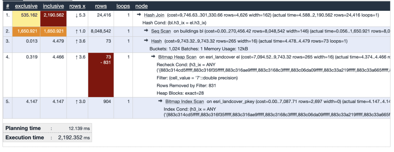
This can further be enhanced if added index on h3_ix column of buildings

create index on buildings(h3_ix);

When shooting count : there were 24416 buildings in my area with built class classified as from ESRI

Verification

Lets verify if the output is true : Lets get the buildings as geojson

WITH t1 AS (
  SELECT *
  FROM esri_landcover el
  WHERE h3_ix = ANY (
    get_h3_indexes(
      ST_GeomFromGeoJSON('{
        "coordinates": [
          [
            [83.72922006065477, 28.395029869336483],
            [83.72922006065477, 28.037312312532066],
            [84.2367635433626, 28.037312312532066],
            [84.2367635433626, 28.395029869336483],
            [83.72922006065477, 28.395029869336483]
          ]
        ],
        "type": "Polygon"
      }'), 8
    )
  ) AND cell_value = 7
)
SELECT jsonb_build_object(
  'type', 'FeatureCollection',
  'features', jsonb_agg(ST_AsGeoJSON(bl.*)::jsonb)
)
FROM buildings bl
JOIN t1 ON bl.h3_ix = t1.h3_ix;

Lets get h3 cells too

with t1 as (
  SELECT *, h3_cell_to_boundary_geometry(h3_ix)
  FROM esri_landcover el
  WHERE h3_ix = ANY (
    get_h3_indexes(
      ST_GeomFromGeoJSON('{
        "coordinates": [
          [
            [83.72922006065477, 28.395029869336483],
            [83.72922006065477, 28.037312312532066],
            [84.2367635433626, 28.037312312532066],
            [84.2367635433626, 28.395029869336483],
            [83.72922006065477, 28.395029869336483]
          ]
        ],
        "type": "Polygon"
      }'), 8
    )
  ) AND cell_value = 7
)
SELECT jsonb_build_object(
  'type', 'FeatureCollection',
  'features', jsonb_agg(ST_AsGeoJSON(t1.*)::jsonb)
)
FROM t1

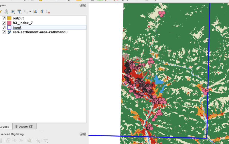
Accuracy can be increased after increasing h3 resolution and also will depend on input and resampling technique

Cleanup

Drop the tables we don't need

drop table planet_osm_line;
drop table planet_osm_point;
drop table planet_osm_polygon;
drop table planet_osm_roads;
drop table osm2pgsql_properties;

Optional - Vector Tiles

To visualize the tiles lets quickly build vector tiles using pg_tileserv

• Download pg_tileserv Download from above provided link or use docker
• Export credentials

export DATABASE_URL=postgresql://postgres:postgres@localhost:5432/postgres

• Grant our table select permission

GRANT SELECT ON buildings to postgres;
GRANT SELECT ON esri_landcover to postgres;

• Lets create geometry on h3 indexes for visualization ( You can do this directly from query if you are building tiles from st_asmvt manually)

ALTER TABLE esri_landcover 
ADD COLUMN geometry geometry(Polygon, 4326) 
GENERATED ALWAYS AS (h3_cell_to_boundary_geometry(h3_ix)) STORED;

• Create index on that h3 geom to visualize it effectively

CREATE INDEX idx_esri_landcover_geometry 
ON esri_landcover 
USING GIST (geometry);

• Run

  ./pg_tileserv

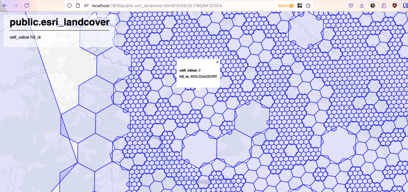
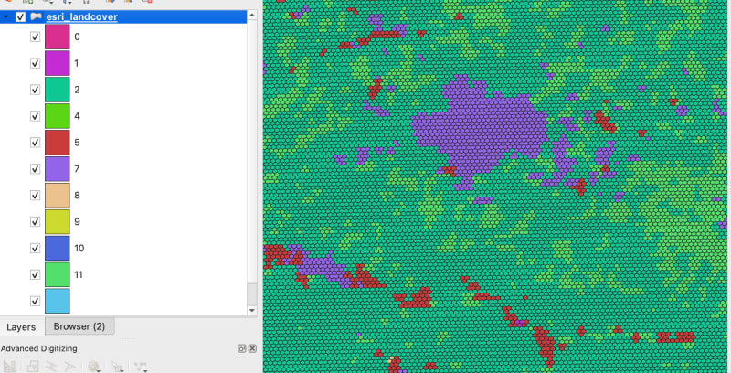
• Now you can visualize those MVT tiles based on tiles value or any way you want eg : maplibre ! You can also visualize the processed result or combine with other datasets. This is the visualization I did on h3 indexes based on their cell_value in QGIS

Source Repo : https://github.com/kshitijrajsharma/raster-analysis-using-h3

References :

• https://blog.rustprooflabs.com/2022/04/postgis-h3-intro
• https://jsonsingh.com/blog/uber-h3/
• https://h3ronpy.readthedocs.io/en/latest/